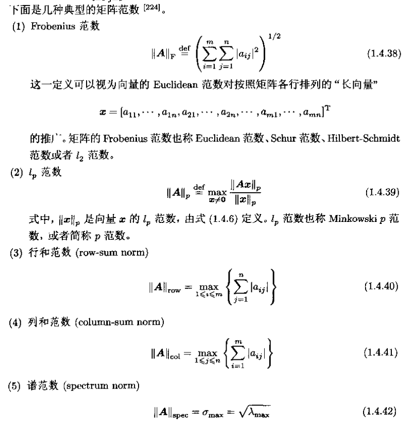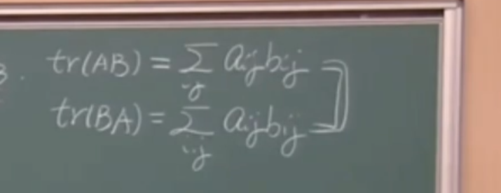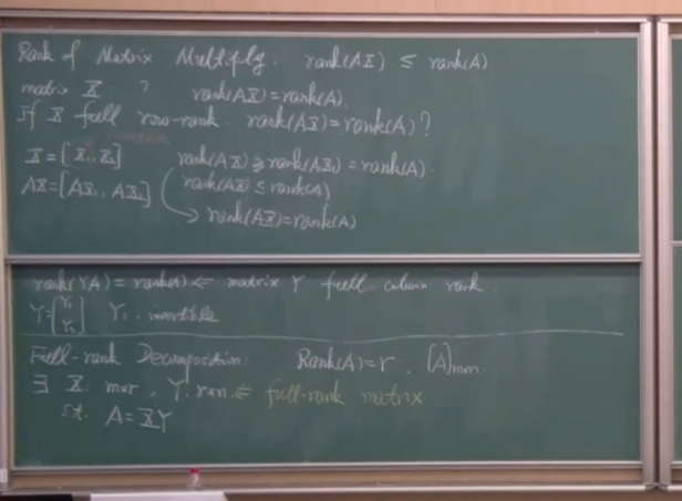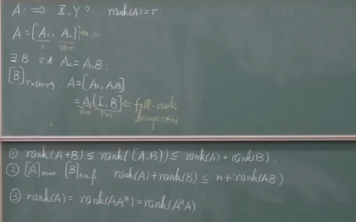
李航之ch3 k邻近法

page39 ~

kd tree page41
3 elements: 距离度量, k值的选择 和分类决策规则

李航之ch1统计学习方法概论

统计学习 监督学习

统计机器学习(statistical machine learning) 建立在计算机及网络之上的, 数据驱动的, 目的是对数据预测和分析的, 构建了模型并且应用模型预测和分析的, 应用到了概率论, 统计学, 计算理论,最优化理论和计算机信息论的.

方法

• supervised learning(*)
• nusupervised learning
• semi-supervised learning
• reinforcement learning

基本概念

输入空间
特征空间= 特征向量存在的空间.每一维度对应一个特征. (有时候这两个空间等同,有时候不一样)
输出空间
联合概率分布
假设空间

统计学习三要素 模型 策略和算法

方法 = 模型 + 策略 + 算法
1 策略, 需要首先损失函数与风险函数的概念, loss 度量模型一次预测的好坏, 风险函数度量平均意义下的模型预测的好坏
2 经验风险最小化与结构风险最小化
经验风险最小化 能保证有很好的学习效果.
结构风险最小化 类似于 最优化.

正则化和交叉验证

指示函数 I
r + e = 1

泛化能力

generalization ability
generalization error (less , better)
generalization error bound (less , better)
function(capacity) 假设空间容量越大,模型就越难学, 泛化误差上界就大
page 15 Hoeffding unequation

生成模型generative model 与判别模型 discriminative

page18 生成方法的特点, 判别方法的特点

分类问题

page19

回归问题

美句

• No matter what happens, he always has an air of detachment.(漠然的样子)

• This preoccupation inevitably leads to an old debate: whether nature or nurture moulds us more.这种关注不可避免地导致了一场熟悉的辩论：天性和后天培养哪一个塑造我们更多。

• These 14 million children most urgently need to develop the resilience that is nurtured with play.这1400万儿童极其迫切需要通过玩耍从而培养他们的韧性

• Aisles of marketing genius belie the fact that, ultimately, weight loss is dictated by the laws of arithmetic.药店过道里的营销天才掩盖了一个事实，即减肥最终是由算术法则决定的。

• There’s not a scrap of evidence to support his claim.没有丝毫证据支持他的说法

真题长难句

• Following the Harvard scandal, Mary Miller, the former dean of students at Yale, made an impassioned appeal to her school’s professors to refrain from take-home exams.

• “It sets such an awful precedent for the future of performance.” Her father, Robin Williams, who died in 2014, was keen to avoid the same fate.

• But a passing reference in a recent profile by Glamour magazine, to her 20-hour workdays prompted an outpouring of admiration.引发了人们的倾佩之情(的倾泻)

• Doing a poor job communicating science to the public will only create confusion and widen the gap between science and society, a gap that scientists are trying to close. (n.困惑，糊涂，迷茫)

• It is text that enables us to uncover lies, confusions and overgeneralizations, and to detect abuses of logic and common sense.正是文本让我们能够发现谎言、混淆和过度概括，并察觉逻辑和常识的滥用。

• One government proposition is to eliminate $10,000 of debt for ‘economically distressed’ students.

• Some UK cities have lobbied without success for the power to levy a charge on visitors.
  一些英国城市为取得向游客收费的权力进行了游说，但没成功。

• It’s Tiffanie Standard, a counselor for young women of color in Philadelphia who want to be tech entrepreneurs — but who must work multiple jobs to stay afloat.
  蒂芙尼·斯坦达德是费城的一位顾问，为那些想成为科技企业家但又不得不身兼数职以求生存的有色人种年轻女性服务。

• We’re allocating too many resources to disciplines that don’t match the needs of employers.
  我们将太多的资源分配到与雇主需求不匹配的学科上。
• But the investigators could not find any data to indicate which species can remember a greater number of distinct human voices, so it was impossible to compare the two on that front.
  但研究人员找不到任何数据来表明哪些物种记住的不同人类声音更多，所以不可能在这方面对两者进行比较。
• For the remainder, the risk of cancer, while increased at the end of life, must be balanced with other factors like remaining life expectancy.
  对于其他人来说，癌症风险在生命晚期可能增加，而其他因素（比如预期寿命）必须综合起来进行考虑。
• Less than half of all American adults were proficient readers in 2017.
  2017年，只有不到一半的美国成年人是熟练的阅读者。

• They give priority to relationships, as careers often recede.
  事业的重要性往往会逐渐降低，他们把处理各种关系放在了重要位置。

• There are queues to climb Mt. Jolmo Lungma as well as to see famous paintings. Leisure, thus conceived; is hard labour, and returning to work becomes a well-earned break from the ordeal.
  人们排着队去攀登珠穆朗玛峰，欣赏名画。如此想来，休闲是一种艰苦的劳动，而重返工作岗位则成了摆脱磨难的一种应有的休息。

• In January 1901, at 1,020 feet, almost precisely the depth predicted by Higgins’ wild guess, the well roared and suddenly ejected mud and six tons of drilling pipe out of the ground, terrifying those present.
  1901年1月，在1020英尺的深处——几乎与希金斯的大胆预测完全吻合——油井轰鸣着，泥浆和6吨重的钻杆突然喷出地面，吓坏了在场的人。

• There appears little prospect of this desperate situation being remedied without radical action being taken.
  在不采取激进行动的情况下，这种绝望的局面似乎不太可能得到补救。

• We received a fast and quick response from the Balinese people. Not only positive responses from the Balinese, we received good responses from the central government, other local governments and even from overseas. Koster told the Sydney Morning Herald this week during an interview.
  在本周的一次采访中，科斯特告诉《悉尼先驱晨报》：“我们从巴厘岛人民那里得到了快速的回应。我们不仅从巴厘岛人那里收到了积极回应，还从中央政府、其他地方政府甚至是海外收获了良好的回应。”

• This criticism may ultimately discourage people from doing good deeds.
  这种批评最终可能会阻碍人们做好事。

  词汇

  recede

  vi. 退，退去，渐渐远去；向后倾斜；缩进；（特点，感觉）逐渐减少；（可能性）变得渺茫

  trench

  n. 沟，沟渠；战壕；海沟

  primary

• adj. 首要的，主要的；最初的；原本的；第一手的, 直接的；初级的, 小学的；初等的

  gorgeous

  adj. 华丽的，灿烂的；令人愉快的

  impair

• vt. 损害，损伤；削弱

peg

• n. 小钉，栓，挂物钉；桩
• vt. 用钉子钉，用钉（或桩等）固定；限定（价格、工资等）；将…看成，将…归入

violate [‘vaɪəleɪt]

• vt. 违反；侵犯，妨碍；亵渎

  volatile [‘vɒlətaɪl]

• n. 挥发物；有翅的动物
• adj. [化学] 挥发性的；不稳定的；爆

benevolence

n.仁爱, 善行, 厚道, 捐助

数学课程

1. 微积分
2. 高等代数(and 矩阵论)
3. 概率论
4. 复分析
5. 凸优化

计算机课程

1. c/c++
2. 算法和数据结构
3. 操作系统
4. 编译原理
5. 计算机网络
6. 数字电路和模拟电路

空闲时间找项目或者赚点小钱

1. python和react 的web 编程
   …

Properties on the Matrix Inverse

Inner Product

$<u,v>$

矩阵的共轭转置

Frobenius 范数

Rank of a Matrix

1. max number of linearly independent rows/cols
2. rank(A) = dim row(A) = dim col(A)

$row(A) = { y^TA}$

这里面其实有A = XY (总可以)

未来我们使用这个性质 就是总可以 AB = XY (if AB!= 0)

determination of MATRIX

properties of det(A)

8 properties AND 2 other properties

how to use java

compile:

1

$ javac hello.java hello

run:

1

$ java hello

1

print('hello world')

hello world

Property 1: The determinant of the identity matrix is one;
Property 2: The determinant changes sign under row/column interchange;
Property 3: The determinant is a linear function of the first row, holding all other rows
fixed.

SVD from EVD

要从矩阵$AA^H$

1. 计算矩阵$AA^H$

   • $U$
   • $\Lambda$

2. 计算矩阵A的奇异值分解（SVD）：
   一旦您获得了矩阵$AA^H$

   • $U$
   • $\sqrt{\Lambda}$
   • $V^H$

因此，基本上，您使用$AA^H$

SVD properties

“MP inverse based on the SVD” 表示基于奇异值分解（SVD）计算的Moore-Penrose伪逆（MP逆）。

奇异值分解（SVD）是一种将一个矩阵分解为三个矩阵乘积的数学工具，具体而言，将矩阵A分解为以下形式：

$A = U \Sigma V^H$

其中：

• U是一个酉矩阵（正交矩阵），它的列包含A的左奇异向量。
• Σ是一个对角矩阵，其对角线上的元素是A的奇异值。
• $V^H$

Moore-Penrose伪逆（MP逆）是矩阵的一种广义逆，可以用来求解线性最小二乘问题以及在矩阵求逆不可行时的一些问题。对于一个矩阵A，它的MP逆通常表示为$A^+$

“MP inverse based on the SVD” 意味着通过使用A的奇异值分解（SVD），可以计算其Moore-Penrose伪逆$A^+$

$A^+ = V \Sigma^+ U^H$

其中，Σ^+是Σ的伪逆，即将Σ的非零奇异值取倒数，然后取共轭转置。

这种方法在数值计算和线性代数中非常有用，特别是在处理奇异矩阵（不可逆矩阵）或求解超定系统（过多未知数的线性方程组）时。

矩阵A的伪逆（Moore-Penrose伪逆）记作$A^{+}$

1. $AA^{+}A = A$
2. $A^{+}AA^{+} = A^{+}$
3. $(AA^{+})^T = AA^{+}$
4. $(A^{+}A)^T = A^{+}A$

现在，考虑$x_0 = A^{+}y$

从$x_0 = A^{+}y$

$Ax_0 = AA^{+}y$

根据伪逆的性质，我们可以将其简化为：

$Ax_0 = (AA^{+})y = y$

因此，如果$Ax_0 = y$

然而，有些情况下这个等式可能不成立：

1. 如果矩阵A是奇异矩阵（不满秩），则可能不存在唯一的y解。在这种情况下，A将没有完整的Moore-Penrose伪逆。

2. 如果$Ax_0$

因此，$y = A^{+}x_0$

The statement you’ve provided suggests that if you have a vector x such that the 2-norm (Euclidean norm) of the difference between A times x_0 and y is equal to the 2-norm of the difference between A times x and y (i.e., ‖Ax_0 - y‖_2 = ‖Ax - y‖_2), then the norm of x_0 is less than or equal to the norm of x (‖x_0 ‖_2 ≤ ‖x‖_2), and equality only holds when x_0 is equal to x.

This statement is related to the concept of the orthogonal projection. When ‖Ax_0 - y‖_2 = ‖Ax - y‖_2, it means that both x_0 and x minimize the 2-norm of the error between the projected vector A times x (or A times x_0) and the target vector y.

In such a case, x_0 and x are both candidates for the solution, but the statement ‖x_0 ‖_2 ≤ ‖x‖_2 implies that x_0 is the solution that minimizes the norm among all possible solutions. If ‖x_0 ‖_2 is less than ‖x‖_2, it means that x_0 is closer to the origin, and therefore has a smaller Euclidean norm.

Equality ‖x_0 ‖_2 = ‖x‖_2 only holds when x_0 is equal to x, indicating that x_0 is the optimal solution. If x_0 is not equal to x, it implies that x is further away from the origin than x_0, resulting in a larger Euclidean norm.

So, when ‖Ax_0 - y‖_2 = ‖Ax - y‖_2, x_0 is the solution that minimizes the 2-norm of the error, and its norm is either less than or equal to the norm of any other candidate solution x.

要证明 $x = A^{+} y$

考虑最小化目标函数：f(x) = ||x||（即，f(x) 是 x 的 2-范数）。

我们有一个等式约束：$x = A^{+} y$

使用 KKT 条件，我们得到以下条件：

1. 梯度条件：∇f(x) - λ(∇(x - A^{+}y)) = 0，其中 λ 是 Lagrange 乘子。

2. 稳定性条件：f(x) 在 x = A^{+}y 处是凸函数。

现在，我们来分析这些条件：

1. 梯度条件：∇f(x) = 2x，∇(x - A^{+}y) = I，其中 I 是单位矩阵。因此，梯度条件变为：2x - λI = 0。

2. 稳定性条件：我们知道 2-范数是一个凸函数，因此 f(x) = ||x|| 在整个定义域上都是凸的。

现在，考虑 Lagrange 乘子 λ 和梯度条件。由梯度条件，我们有：

2x - λI = 0

这意味着 x = (1/2λ)I。

现在，我们回到我们的目标函数 f(x) = ||x||。根据 x 的表达式，我们有：

f(x) = ||(1/2λ)I|| = (1/2λ)||I|| = 1/(2λ)

因此，我们看到当 λ 取得最小值时，f(x) = 1/(2λ) 取得最大值。这意味着我们要最小化 ||x||，必须使 λ 取得最小值。而根据 KKT 条件，λ 必须是非负的。因此，λ 最小值为 0。

当 λ = 0 时，我们得到 x = (1/2λ)I = (1/2*0)I = 0I = 0。这表明 x = A^{+}y 是 ||x|| 的最小解，因为它使目标函数取得最小值 0。

因此，我们已经证明 x = A^{+}y 是 ||x|| 的最小解。

设 X_1, …, X_n 是从正态分布 $N(\mu, \sigma^2)$

要进行假设检验问题 H0: σ = σ0 vs. H1: σ ≠ σ0，你可以仿照 Wald 检验，但使用卡方分布来替代标准正态分布，具体的步骤如下：

1. 提出原假设 (H0) 和备择假设 (H1)：

   • 原假设 (H0): σ = σ0
   • 备择假设 (H1): σ ≠ σ0

2. 收集样本数据，计算样本标准差 (s)。

3. 计算检验统计量 (Wald 统计量)：

   • Wald 统计量的计算方式为：
     W = [(n - 1) * s^2] / σ0^2
     其中，n 是样本容量，s 是样本标准差，σ0 是原假设中的标准差。

4. 基于卡方分布 (χ^2) 进行检验：

   • 在这个情况下，Wald 统计量 W 满足自由度为 n - 1 的卡方分布，即 W ~ χ^2(n - 1)。

5. 选择显著性水平 (α).

6. 根据所选择的显著性水平 (α) 和自由度 (n - 1) 查找卡方分布表格或使用统计软件，确定卡方临界值 (χ^2_critical)，使得 P(χ^2 > χ^2_critical) = α/2。

7. 判断是否拒绝原假设:

   • 如果 W > χ^2_critical 或 W < 1 / χ^2_critical，则拒绝原假设 (H0).
   • 如果 W ≤ χ^2_critical 并 W ≥ 1 / χ^2_critical，则无法拒绝原假设 (H0).

8. 根据判断的结果，得出对标准差 σ 的结论:

   • 如果拒绝原假设，说明在所选显著性水平下，有足够的证据表明标准差 σ 不等于 σ0.
   • 如果未能拒绝原假设，说明在所选显著性水平下，没有足够的证据表明标准差 σ 与 σ0 不同。

这样，你就可以使用卡方分布来进行关于标准差 σ 的假设检验，检验是否存在显著差异。

To prove that for any non-singular matrix A, there exists an upper-triangular matrix T such that TA is a unitary matrix, we can use the concept of the QR decomposition.

QR decomposition decomposes any matrix A into a product of two matrices: Q (orthogonal or unitary) and R (upper triangular). Specifically:

A = QR

Here, Q is unitary, and R is upper triangular.

Now, let’s prove the statement for a non-singular matrix A:

1. Given a non-singular matrix A, perform the QR decomposition:

   A = QR

   Here, Q is unitary, and R is upper triangular.

2. We want to show that TA is unitary:

   TA = TQR

3. Since Q is unitary, we have:

   Q^H Q = I

   (Where Q^H is the conjugate transpose of Q, and I is the identity matrix).

4. Now, let’s define T = Q^H. Since Q is unitary, we have:

   T = Q^H

   Then, TA becomes:

   TA = (Q^H) QR

5. Since T = Q^H and Q^H Q = I, we have:

   TA = IR

6. Any upper triangular matrix multiplied by its own conjugate transpose (in this case, R and R^H) will result in the identity matrix times a unitary matrix (IR), which is unitary itself.

So, TA is a unitary matrix, and we have successfully shown that for any non-singular matrix A, there exists an upper-triangular matrix T (in this case, T = Q^H) such that TA is a unitary matrix.

Prove : If A is a real matrix, and $A + A^T = 0$

Let $A$

$P_A(x) = \det(A - xI)$

We want to show that $P_A(A) = 0$

Substituting $x$

$P_A(A) = \det(A - AI)$

Now, we use the properties of determinants:

$\det(A - AI) = \det(A(I - A))$

We can factor out $A$

$\det(A(I - A)) = \det(A) \det(I - A)$

Since $A$

$\det(A) \cdot c$

We need to show that $\det(A) \cdot c = 0$

Since $c$

Now, we have:

$\det(A) \cdot c = \det(A) \cdot c^n$

We know that the determinant of a matrix raised to its order is always zero (if it’s not invertible):

$\det(A^n) = 0$

Therefore, we have:

$\det(A) \cdot c = 0$

This concludes the proof that Hamilton-Cayley theorem holds:

$P_A(A) = \det(A - AI) = \det(A) \det(I - A) = \det(A) \cdot c = 0$